Simulation pipeline#
Our Myoelectric Digital Twin is a cloud based software with a Python API which allows users a simple yet flexible way to define various simulation parameters and to control the simulation pipeline. User can define subject’s anatomy, different tissue conductivities, the electrode configuration, individual fiber properties, motor unit and recruitment model parameters, as well as the activations of each muscle, etc.
The following figure shows a schematic representation of the user’s inputs, main simulation modules and their interaction.
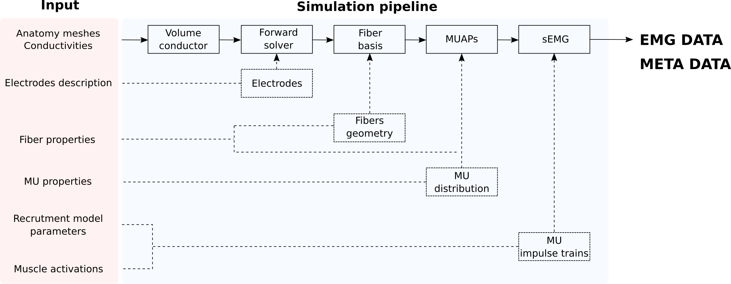
Some of the objects present in the simulation pipeline have clear physical or physiological meaning (volume conductor, fibers, etc.), and some of them are rather abstract and contain the information required for the computation (forward solver, fiber basis)
Each step of the simulation pipeline depends on the output of the previous module and on a specific subset of the input parameters. This hierarchical architecture, dictated by the mathematical properties of the model, allows efficient management of pre-computed data (i.e. changing fiber properties does not require recomputing the forward solver).
The mathematical details can be found in our paper Towards the Myoelectric Digital Twin: Ultra Fast and Realistic Modelling for Deep Learning.
We will now introduce all the main computational steps of the simulation pipeline in details.
Volume conductor#
Volume conductor is an object that contains:
Tetrahedral volume mesh representing the discretized anatomy. Each tetrahedron contains specific domain label (e.g. individual muscle id) and corresponding tissue type (bone, muscle, fat, skin, electrode).
Conductivity tensors are defined for each tetrahedron.
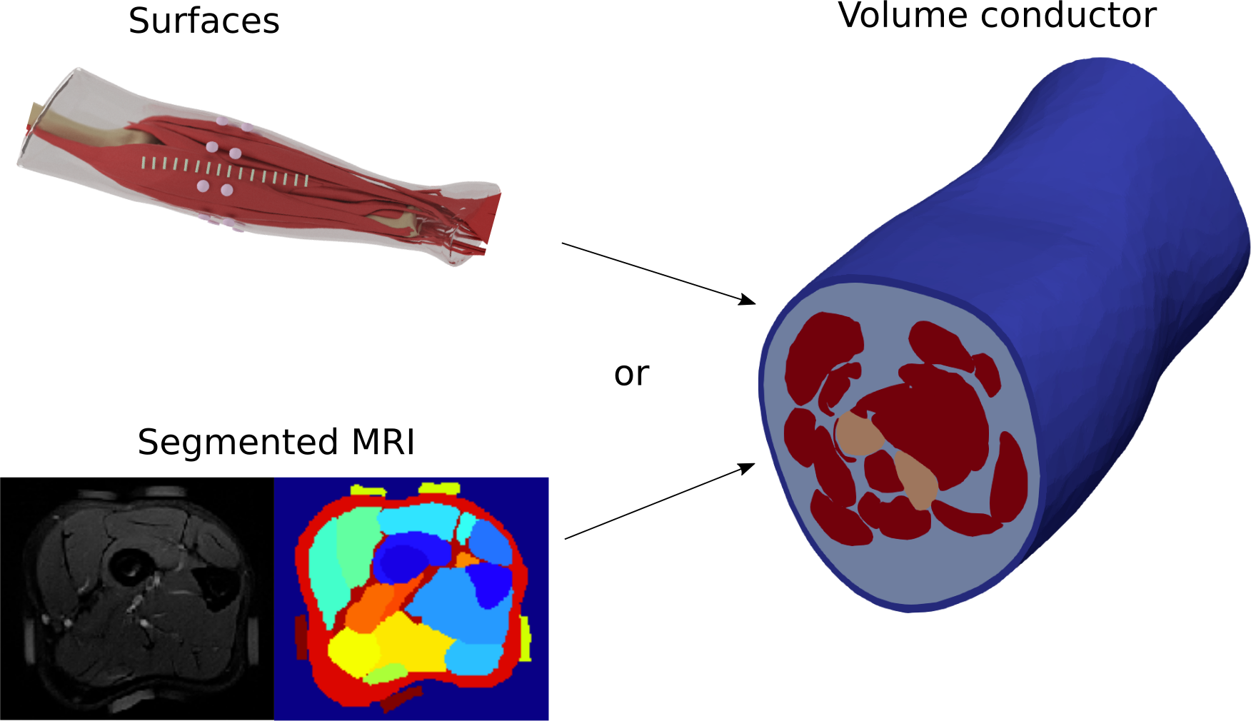
The volume conductor can be generated either from surface meshes or from segmented MRI (will be added to the API soon). As for the conductivity tensors, user only has to define it for each tissue type - tensors for each tetrahedron will be assigned automatically. Note, that muscle conductivity is anisotropic, and the tensor’s main direction is automatically chosen to follow the muscle geometry.
Associated API: mdt.Conductor
Electrodes#
Electrodes description should be provided to compute EMG data.
One way to introduce it is by providing surface mesh for each electrode (with corresponding tissue type) as an input for the volume conductor. In this case, forward solver (see next section) will be computed for the corresponding skin-electrode interfaces.
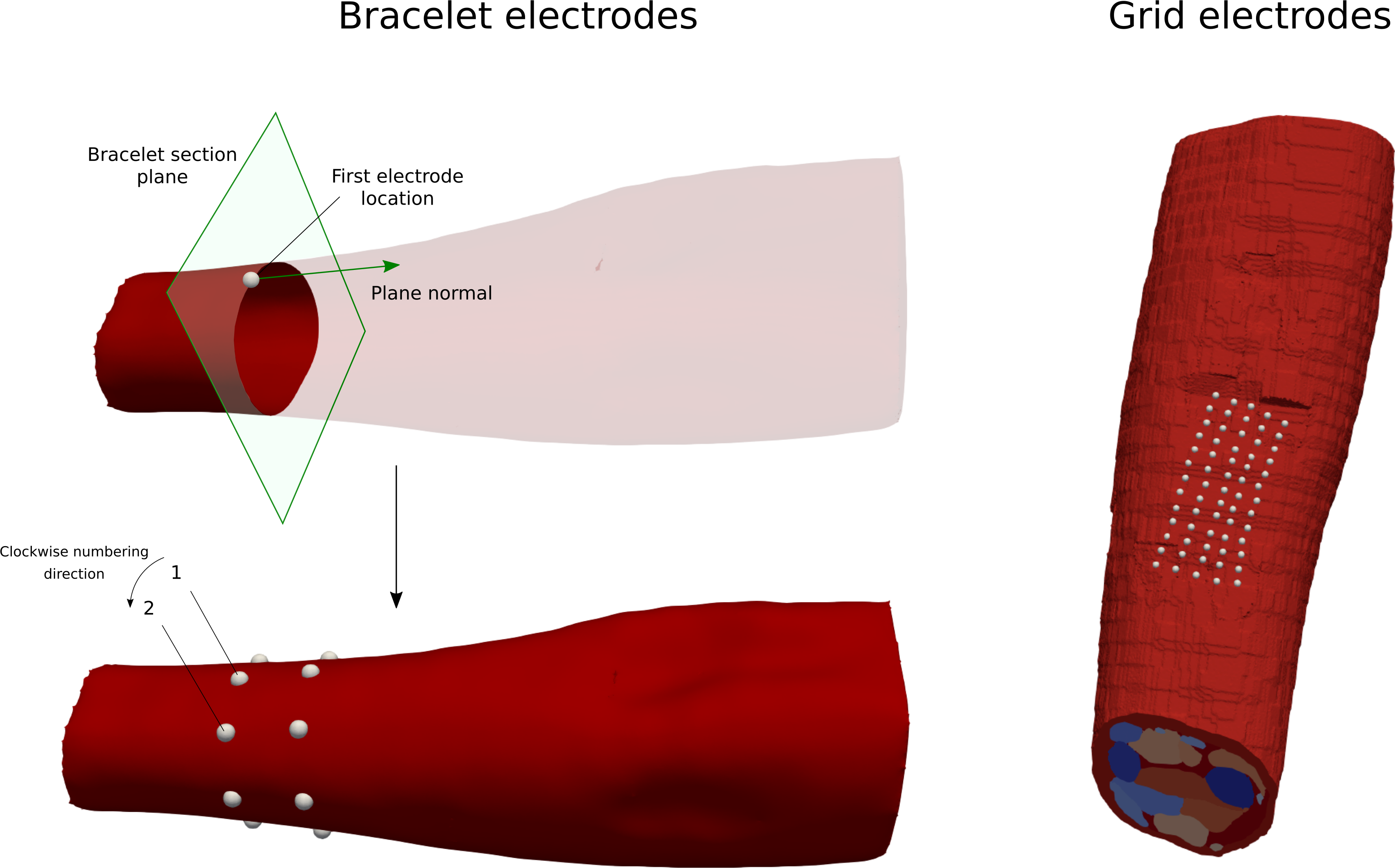
Another way to describe the circular electrodes is by providing their center locations and radii. We provide functions that allow automatically generate bracelet and grid (will be added to the API soon) electrode configurations.
Associated API: mdt.Electrode, mdt.ElectrodeBracelet
Forward solver#
Forward solver is an object that contains “general solution” of Poisson equations for the specific volume conductor and electrode configuration. The mathematical details can be found in our paper, but from the user’s perspectives the takeaway points are:
Forward solver only depends on volume conductor (mesh and conductivities) and electrode configuration. Thus, changing one of those parameters will require recomputing of the forward solver. Recommendation: if you want to simulate multiple electrode configurations, you may concatenate them into a single one, and then decompose the resulting EMG signal into separate configurations.
Computational time depends linearly on the number of electrodes.
Forward solver does not depend on the fibers and motor units geometry and properties, thus changing those parameters does not require recomputing it.
Associated API: mdt.ForwardSolution
Fibers and fiber basis#
The next step is to generate fibers geometry for each muscle of interest. We provide a function that does it automatically based on the muscle geometry.
User can directly input the number of fibers for a given muscle, or it can be automatically estimated from the muscle cross-section area and the average fiber radius (provided by user)
Our approach consists in generating a uniform fiber distributions inside a unit circle, “morphing” it into sequence of the muscle cross-sections and thus constructing 3D fiber paths that follow the muscle shape.
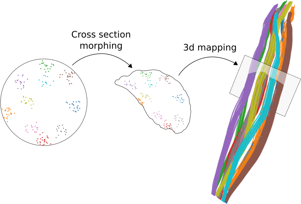
Currently, the planes of the first and the last muscle slices that are used for fiber generation should be provided by user. Each plane is defined by its normal vector and a point that it passes through (an origin point).
The generated fibers will start at the first plane cross-section, follow the muscle geometry and finish at the second plane cross-section.
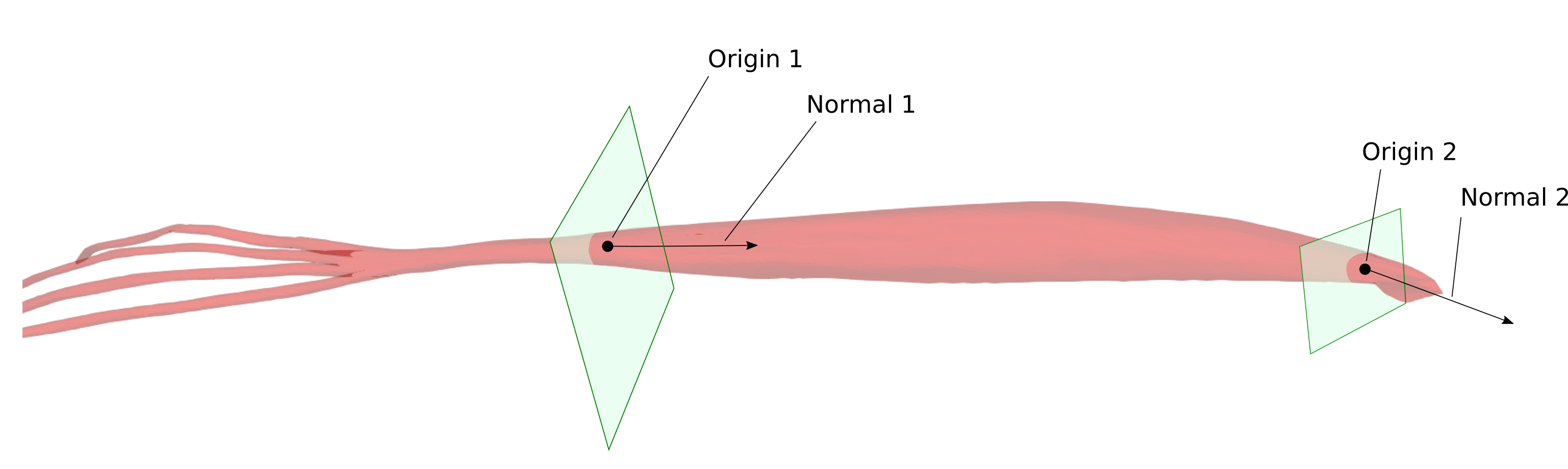
The selection of those planes will be automated soon.
Associated API: mdt.Fibers
Once the fibers geometry is generated for a muscle, we need to “project” the general forward solver to those fibers. Corresponding object is called fiber basis. It is computed for each muscle of interest and it depends on a specific forward solver and corresponding muscle fibers geometry. Thus, it will be recomputed if and only if some of those inputs is altered. Fiber basis does not depend on motor units distribution and fiber physiological properties.
Associated API: mdt.FiberBasis
Fiber properties#
There is a set of parameters that can be defined for each muscle fiber:
The relative lengths of tendons (tendon 1 and tendon 2 ratios, value between 0 and 1). This value is with respect to the whole fiber length.
The relative location of neuromuscular junction (value between 0 and 1). This value is with respect to the length to the active fiber (i.e. excluding the tendons)
The action potential propagation velocity (m/s)
Our API allows defining minimum and maxim parameter values for a muscle. The individual fiber parameters will be then randomly assigned following the uniform distribution between those bounds.
Associated API: mdt.FiberProperties
Motor unit distribution#
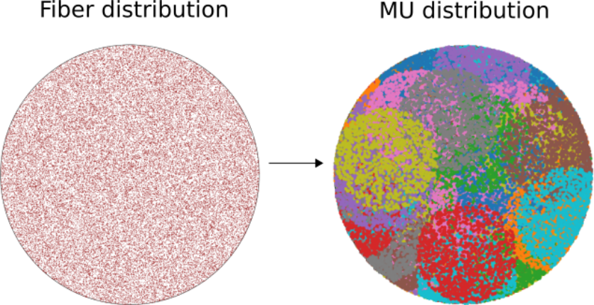
For a given fibers geometry and corresponding distribution inside a unit circle, those fibers are then randomly grouped into motor units (MUs). Our model has the following properties:
MU centers are uniformly placed inside the unit circle.
MU size (i.e., number of fibers per MU) distribution has exponential form - a lot of small ones, few large ones. See this paper for details.
User can define the range of the relative MU territory areas, i.e., percentage of the cross-sectional area of a muscle occupied by individual motor units. The default range of the areas is between 10% and 70%.
Each fiber belongs to one and only one MU.
Associated API: mdt.MotorUnits
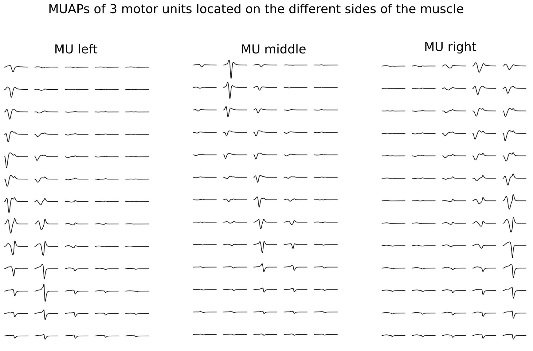
Motor unit action potentials (MUAPs)#
Now we have all the elements to compute the EMG signal at each electrode associated to each motor unit when it receives an impulse from a motor neuron. This signal is called motor unit action potentials (MUAPs). The model assumes, that all the fibers of a motor unit are activated simultaneously. Thus, MUAP for a given motor unit is a superposition of the electric potentials generated by each fiber of this MU.
For a given fiber and electrode, the corresponding EMG signal is computed as an integral of the forward solution and a current source density (CSD) along the fiber. Forward solution is stored in the fiber basis object, and thus depends on the volume conductor, electrodes location and fiber geometry. CSD is a function of the physiological fiber parameters and of the desired time sampling frequency.
Note: the resulting MUAPs have an average electrode montage. It means that for each time sample, the average of the EMG signal over all the electrodes is zero.
Associated API: mdt.MotorUnitsActionPotentials
Impulse trains and assembled EMG#
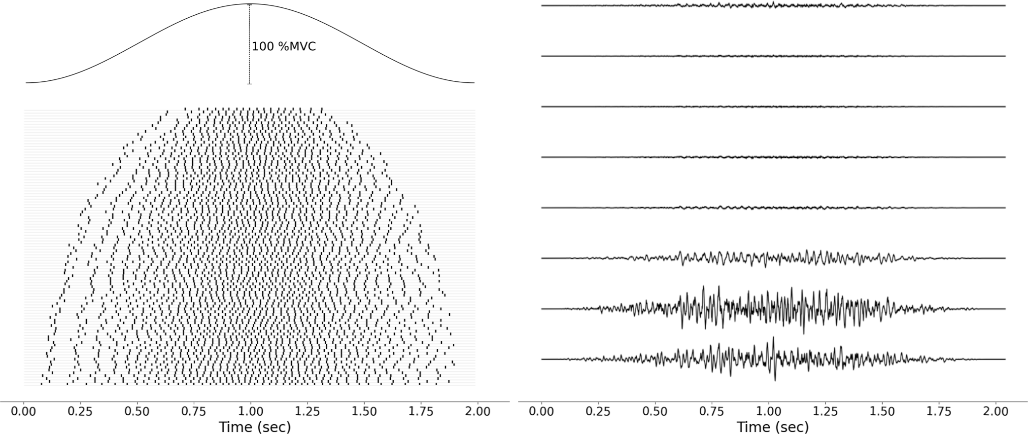
The magnitude and direction of the force exerted by a muscle depends on the number of motor units that are activated (recruitment) and the rates at which they discharge action potentials (rate coding). Motor units tend to be recruited in a relatively fixed order during voluntary contractions. The orderly recruitment of motor units follows the size principle in which small motor neurons are recruited before progressively larger motor neurons.
In our model user needs to provide an activation pattern for a given muscle - percentage of maximum voluntary contraction (%MVC) as a function of time. This input is then decomposed into impulse trains for ech MU of the muscle. This decomposition is largely based on this paper and follows the following principles:
Smaller MUs are recruited before large ones (size principle).
Recruited MUs linearly increase their firing rates with increasing %MVC until it reaches a certain maximum.
There is an upper limit of motor unit recruitment, i.e. the value of %MVC all the muscle MUs are recruited
Once the impulse trains are constructed for each MU, they are combined with their MUAPs to assemble the sEMG signal corresponding to the given muscle activation. The sEMG signal is computed for each muscle separately and then summed up to get the final raw sEMG data.
The following figure shows how a 2 second long muscle excitation is decomposed into impulse trains for each motor unit, and then assembled into raw sEMG signal.
Associated API: mdt.ImpulseTrains, mdt.Electromyography